hecto, Chapter 6: Search
Table of Contents
- Introduction
- Chapter 1: Setup
- Chapter 2: Entering Raw Mode
- Chapter 3: Raw Input and Output
- Chapter 4: A Text Viewer
- Chapter 5: A Text Editor
- Chapter 6: Search 📍 You are here
- Chapter 7: Syntax Highlighting
- Appendices
- Change Log
Chapter 6: Search
Our text editor is done - we can open, edit and save files. The upcoming two chapters add more functionality to it. In this chapter, we will implement a minimal search feature.
For that, we’re going to reuse our ability to prompt the user for input. This is - at least in my code - currently tightly coupled to the Save-As functionality, so the first task is to prepare our code.
Assignment 26: Search Prompt
- Add a new prompt to open on
Ctrl-F. The basic functionality should be the same as forSave As, with the following differences:- Hitting
Enteron that prompt shouldn’t do anything yet, we’re going to implement the search functionality later. - Instead of showing
Save as:, the prompt should showSearch:
- Hitting
- The initial status message we show to the user should be amended to read:
HELP: Ctrl-F = find | Ctrl-S = save | Ctrl-Q = quit - If applicable, your code should be cleaned up to be able to handle both types of prompt.
Code Review: Here’s how I solved it.
Assignment 27: Preparing for Search
Depending on what your code looks like, most of this assignment might not be needed for you.
Let me explain the big picture first.
To implement a search, our strategy will be to use find , on String. This will return the byte index of the first character of this string. In order to translate this into a location within the text, we will need to find a way to map the byte index to a grapheme cluster.
Achieving that is not hard - unicode_segmentation offers a method called grapheme_indices which returns the byte index alongside the grapheme cluster, as documented here.
However, our (or at least my) data structure to represent a Line is no longer suitable. We built it up coming from the requirements around a text viewer, therefore the data structure is optimised for displaying - it’s basically a vector of layout information - but not for editing, saving or searching, since all these operations require rebuilding the entire string within the current structure. Editing even goes a bit further, an edit operation builds up the entire string, only to rebuild the entire internal structure again and then discard the new string again.
What we should be doing instead is to keep the string around and modify it directly on edit operations - the byte indices returned by grapheme_indices can help us with that. Then, we can discard the internal structure and keep the string around. A Search operation would then directly work on the string without the need to assemble it in the first place.
Here is the assignment:
- Refactor your code to keep a
Stringaround for each line. - Refactor your code to store the
byte_indexfor each fragment - Refactor your code to directly modify the
Stringfor edit operations
Code Review: Here is how I did it.
Assignment 28: Simple Search
Let’s build a first version of our search. Each time a user updates the search query, we will iterate over all rows until we find a match in one of them. We will then scroll the view to that position.
For the first few steps, I recommend that you ignore grapheme clusters. Testing them will be difficult until we have highlighting the results in place.
For the remaining assignments, you can use this file as a test file for your search.
Here is the assignment:
- While the user types in the search prompt, find the first occurrence of the given string from the top and scroll to it. You can iterate over each line to find the correct line index, and use find in each line to find the right byte index, which then needs to be converted to the correct grapheme index.
- If no match is found, don’t do anything.
- If the user leaves the search by hitting Enter, ensure the user can continue editing at the position of that match.
- If the user dismisses the search by hitting
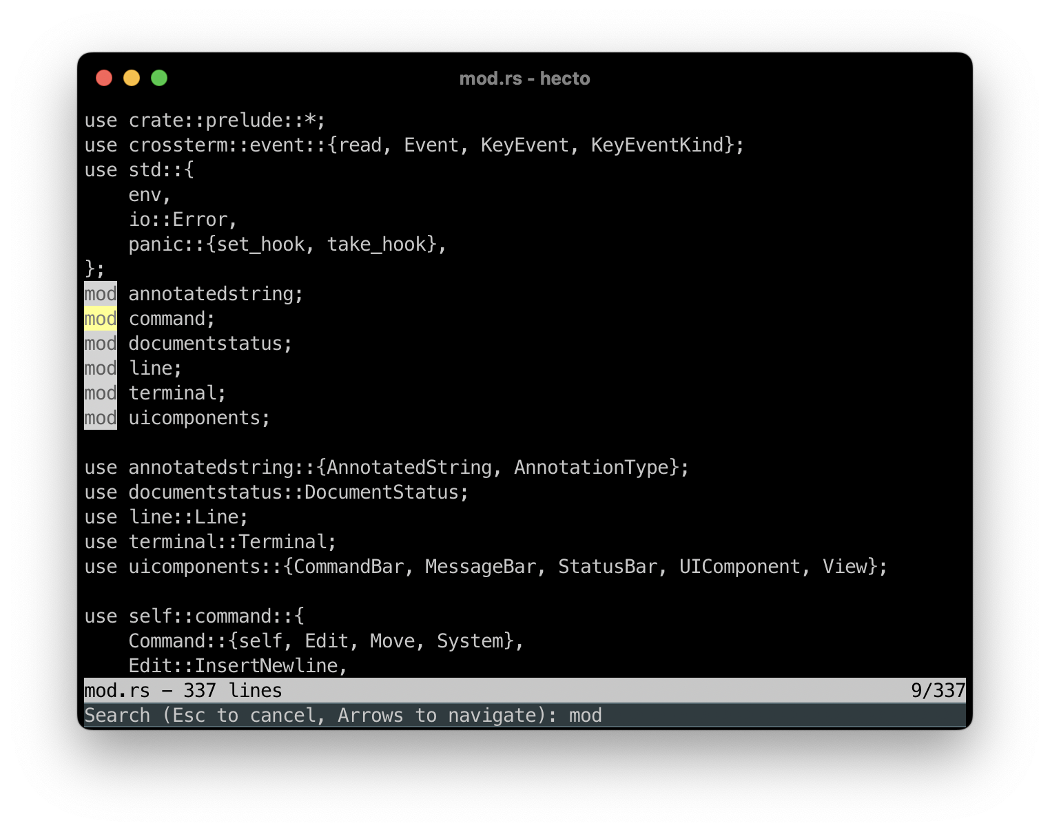
Esc, restore the previous caret position within the text and scroll to it. - Amend the prompt text to read
Search (Esc to cancel):
Code Review: Here is my code.
Assignment 29: Improved Search
Let’s allow navigating through the search results and make our current search a bit more convenient.
Here is the assignment:
- Instead of searching from the top, the search should start from the current position onwards. Finding from a position within a string is equivalent to finding in the slice of that string starting at the desired position.
- Wrap around to the top of the document and search from there until the current location in case no match was found.
- Scrolling to a match should center the match on the screen, to make it more clearly visible.
- Dismissing the search with
Escshould restore the old scroll position exactly instead of just scrolling to the location of the old text position. - Amend the prompt to read:
Search (Esc to cancel, Arrows to navigate): - -> or ↓ should find the next occurrence of the search query after the current match.
Assignment 29: Code Review
Let’s now discuss two aspects which I have raised in my own code. Here’s the first one, extracted into a Rust Playground and simplified:
 pub fn print_hello(show_name: bool) {
        let hello_msg;
        if show_name {
            hello_msg = "Hey Philipp!";
        } else {
            #[cfg(debug_assertions)]
            {
                panic!("Attempting to say hello without using my name!");
            }
            #[cfg(not(debug_assertions))]
            {
                return;
            }
        }
        println!("{hello_msg}");
    }


fn main() {
    print_hello(true);
    print_hello(false);
}
My questions were:
- Why is the return wrapped in a
cfg? - What happens if you remove the whole block, including
return?
Play around with it and try it out.
The first question was already answered in an earlier code review: If we remove the surrounding cfg, clippy assumes that the return is dead code and therefore complains.
The second question can be answered with: Nothing, at first glance. Remove the entire block with #[cfg(not(debug_assertions))], and it works. You’re not getting an error, or a warning.
However, I told you in the annotated commits that the uninitialised use of hello_msg (in this case, in the code review it was step_right) was allowed only because Rust could infer that under no circumstances, show_message was used without being initialised. And it’s true - for debug builds.
But once you switch from Debug to Release (on the top-right on Rust Playground), it won’t compile any more, due to hello_msg being possibly undefined.
Both of these aspects are related to clippy linting for the Debug build only.
To make clippy lint for release, call it like this:
cargo clippy --release
Proper Search Result Navigation
Here’s the second aspect I raised during Code Review:
When navigating to the next search result, we do so by moving the start location just behind the current match and continue searching from there. And I was asking: Why didn’t we just move one step to the right, and save all the logic to determine the length of the search query?
The answer lies with how searches work in other text editors and is concerned with overlapping search results.
Consider the following string: ababa. Your search query is aba, and therefore, you match the first three letters of that string: ababa . If you proceed with the search one step to the right, placing the start position between the a and the baba, would then match the second aba: ababa. That’s not how search usually works - try it out on this page by searching for aba!
This makes sense if you start considering search result highlighting, and features like search-replace into the mix. Searching for aba and highlighting ababa would be strange. Attempting to replace all occurrences of aba with abc would lead to ambiguity: Should the result be abcba? abcbc? ababc?
This will pose an interesting challenge in the next assignment.
Assignment 30: Backward Search
Now, let’s allow the users to search the search direction. Using ↑ or ← should search the previous search result. The simple way to do so would be to use rfind, which works like find, but backwards (documentation here). However, this breaks user expectations, because even on backward search, usually only the first part of overlapping matches should be considered!
An alternative is to use match_indices, which returns an iterator over all matches (starting from the beginning of the string), and which handles overlaps as expected. The documentation is here.
Searching backwards and upwards does not require taking a “step left” prior to searching.
Here is a Rust Playground illustrating several ways to search within a string:
fn main() {
    let needle = "aba";
    let haystack = "ababababa";
    // This haystack contains the needle 4 times
    // at the following indices: 0, 2, 4, 6

    dbg!(haystack.find(needle).unwrap()); //finds the first occurence
    dbg!(haystack.rfind(needle).unwrap()); //finds the last occurence
    for (index, _) in haystack.match_indices(needle) { //Finds the first and third occurence
        dbg!(index);
    }
    for (index, _) in haystack.rmatch_indices(needle) { //Finds second and fourth occurence
        dbg!(index);
    }
    let mut i = 0;
    while let Some(relative_index) = haystack[i..].find(needle) { //Finds all occurences.
        dbg!(relative_index + i);
        i += relative_index + 1;
    }
}
Here is the assignment:
- Pressing ↑ or ← should search backwards for the given query.
- Symmetrical to forward search, the search should wrap around to the bottom if no result has been found.
- Take care of overlapping results, as discussed above.
- Extending the query by continuing to type should not change in behaviour: Searching for the updated string proceeds downwards.
- Check
clippyfor potential warnings forreleasebuilds and fix them where appropriate.
Code Review: Here is my code.
Colors
Our search works! However, using it is not very convenient: If multiple matches are close to ne another, it’s hard to guess which one we’ve currently found. Let’s try and solve this by highlighting it nicely.
To do so, we need to talk about colours, first.
While styling our status bar, we’ve already briefly touched upon the subject, but all we did was invert the current colours, which is, if you think about it, not really using colours at all.
We met the American National Standards Institute, ANSI, already in one of the early chapters - they were the ones who standardised the Escape Codes we’ve been using to set up our terminal.
They also defined a list of eight colours (3 bit) which, could be used to color text output in terminals. These colours are:
- Black
- Red
- Green
- Yellow
- Blue
- Magenta
- Cyan
- White
The following program, which - for obvious reasons - doesn’t work on Rust Playground, prints out these 8 colours:
fn main() {
    for i in 0..7 {
     print!("\x1b[3{};4{}m ",i,i);
     print!("\x1b[0m ");
    }
    println!();
}
\x1b[3{};4{}m sets the foreground color (30-37) and the background color (40-47) to the same value, resulting in the following space being rendered as one block in the target color.
\x1b[0m resets the terminal, resulting in the following space being rendered as empty.
These 8 colours were soon amended by another bit, signalling their “bright counterparts”, which use the codes 90-97 for the foreground, and 100-107 for the background color, respectively.
This is how to print them:
fn main() {
    println!("R B");
    for i in 0..7 {
     print!("\x1b[3{};4{}m ",i,i);
     print!("\x1b[0m ");
     print!("\x1b[9{};10{}m ",i,i);
     print!("\x1b[0m\n");
    }

}
As you can see, the presence of White, Bright White, Black and Bright Black lead to 4 different grey scales being available.
From 4-Bit to RGB
Technology marches on, and soon the 4-bit colours above were extended to 8-bit colours, with a whooping 256 different colours.
Instead of adding more escape codes per color behind the code range 10x for bright background colours, the codes 38 and 48, which were unused because the original 4-bit colours ended at 37 and 47, respectively, were used, with another parameter (5) to indicate the 8-bit color mode.
This is how to print all of them:
fn main() {
    for i in 0..255 {
        print!("\x1b[38;5;{};48;5;{}m ", i, i);
        print!("\x1b[0m ");
    }
}
If you run this, you can see that
- The first 8 colours are the original 8 colours from above
- The next 8 colours are their bright counterparts
- This is followed by 216 other colours
- The last block are 24 grayscales from dark to light.
The next leap after this was RGB, which gives us a couple more colours to use. But before we go there, let’s talk about color conventions.
Color Conventions and Naming
When we talk about colours in the context of software engineering, we usually fall back to color codes instead of referring to the colours by name. Back when there were only 8 colours available, precision did not matter, and it was much more common to refer to the colours by name. In the list of the 8 colours above, there is absolutely no ambiguity to the term “blue”, as there is only one shade of blue available. Which kind of blue actually was rendered could, and did, differ from machine to machine - as I said, precision did not matter too much.
Interestingly, you can see that already the leap from 3 to 4 bit colours made the naming convention fall apart: Suddenly, there was “white” from the 3-bit palette, and the addition brought “Bright White”… which resulted in “white’ being demoted to grey, and Bright White being, well, white.
As an additional example of the delightful mess named colours are, consider this: Did you ever wonder why in CSS, dark grey is actually lighter than grey? If not, now you probably do.
The X Window System, a graphical user interface for Unix-like operating systems, contained a list of mapping color names to their RGB Values (we’ll properly meet RGB soon!). The first browsers used these colours for their mappings. The W3C, which standardised the colours in CSS, used the colours from X11, amended, and in parts overridden, by their own definitions.
Crucially, the W3C definition of “grey” and “light grey” were much darker than the X11 counterparts. However, W3C did not define a “dark grey” variant - so the lighter X11 variant was not overridden and stayed.
Even though my LLM wants me to believe that it’s much more convenient to refer to colours by their name, I have never ever seen a professional context where named colours were used. Instead, we usually use the RGB Color Codes.
RGB and RGB Color Codes
I’m sure that you have used, or at least seen, these codes before. There is, which is close to Coca Cola Red, , which is called Barbie Pink, and my current employer, Zaando, uses for its brand.
But what do these codes mean? These codes are triplets in hexadecimal - in case of Zalando, there is FF, then 69, then 00. In hexadecimal, each digit represents one of 16 values (0,1,2,3,4,5,6,7,8,9,A,B,C,D,E,F). Two digits therefore can represent 16x16=256 values. The first two digits represent the intensity of red, the middle two green and the last two blue - R,G,B.
Additive and subtractive color models
Let’s build up our understanding on color models by simultaneously learning about two color models - RGB, which is typically used for screens, and CMYK, which is used for print.
For the first model, imagine that you are in a completely dark room - it’s pitch black. You have three torch lights with you - one in red, one in green and one in blue. Each torch light has 256 settings - from off to fullest intensity.
For the second model, imagine you are in a well lit room, a piece of empty, white canvas in front of you. You have three ink colours available: Cyan, Magenta and Yellow (the first letter of each of these form the first part of the name of this model: CMYK. We get to the K in a second.)
In the first model, no light hits your retina - it’s completely dark. In the second model, lights of all wavelengths hits your retina - you perceive it as white.
Now let’s take both models to the extreme. In your dark room, turn on all three lights at the same time, all the way from 0 to 255.
Actually, let’s do that in code:
fn main() {
    for i in 0..255 {
        print!("\x1b[38;2;{i};{i};{i};48;2;{i};{i};{i}m ");
        print!("\x1b[0m ");
    }
}
What we do here is that we use almost the same escape code as before, but we switch from color mode 5 (8 bit color mode) to color mode 2 (RGB color mode) and provide the values for Red, Green and Blue separately. Since we want to crank up all three torchlights at the same time, we pass the same value for all three colours - and we do the same for the foreground and background color.
What you can see is grey - all the way from black via almost black, then across all shades of grey to pure white: The mixture of red, green and blue at fullest intensity is sufficient to be perceived as white.
Conversely, if you paint all three colours in the same amount on your canvas - Cyan, Yellow and Magenta - the result will be an increasingly darker shade of grey until you arrive at black.
In theory, or in the perfect world of your mental model, at least. In reality, inks are impure and imperfect, and therefore, the best you will achieve will be some kind of dark brownish color. That’s why in print, black is specifically added as a separate color - referred to as Key, forming the K in CMYK.
Now, let’s mix a few colours - first in the RGB model, by only operating two torchlights at the same time. Let’s also do that in code:
fn main() {
    print!("Red:\t\t");
    print!("\x1b[38;2;255;0;0;48;2;255;0;0m ");
    print!("\x1b[0m ");
    println!();
    print!("Green:\t\t");
    print!("\x1b[38;2;0;255;0;48;2;0;255;0m ");
    print!("\x1b[0m ");
    println!();
    print!("Blue:\t\t");
    print!("\x1b[38;2;0;0;255;48;2;0;0;255m ");
    print!("\x1b[0m ");
    println!();
    print!("Red and Green:\t");
    print!("\x1b[38;2;255;255;0;48;2;255;255;0m ");
    print!("\x1b[0m ");
    println!();
    print!("Green and Blue:\t");
    print!("\x1b[38;2;0;255;255;48;2;0;255;255m ");
    print!("\x1b[0m ");
    println!();
    print!("Red and Blue:\t");
    print!("\x1b[38;2;255;0;255;48;2;255;0;255m ");
    print!("\x1b[0m ");
    println!();
}
What you can see is that:
- Red and Green produces Yellow
- Green and Blue produces Cyan
- Red and Blue produces Magenta
Magenta is a very interesting case: Yellow, Cyan, Red, Green and Blue are “Colours of the Rainbow”, meaning that all of these colours have a spectrum of wavelength assigned to them. Magenta, on the other hand, mixes, as we just saw, Red and Blue, which are pretty far apart on the visible spectrum , but the brain interprets it as a distinct color.
RGB is an additive color model, because we start with black and add colours and intensity (like red and green to produce yellow) until we’ve created the color we wanted.
Let’s apply this knowledge to the CMYK model. Our Yellow ink reflects only Red and Green (as we’ve seen above: red and green light produces yellow), and our Cyan ink reflects only Green and Blue. If we mix them, the mixture absorbs everything except green (which is reflected by both inks) - so Cyan and Yellow results in Green. Similarly, Cyan and Magenta produces blue, and Magenta and Yellow produces Red.
CMYK is a subtractive color model, because we start with white and take away colours and intensity (like Cyan and Yellow absorbed everything except Green) until we’ve created the color we wanted.
Since any of the two triplets - Cyan, Yellow, Magenta and Red, Green, Blue, can create the other one, they can create an equivalent set of colours.
Let’s print them all!
fn main() {
    for r in 0..255 {
        for g in 0..255 {
            for b in 0..255 {
                print!("\x1b[38;2;{r};{g};{b};48;2;{r};{g};{b}m ");
                print!("\x1b[0m ");
            }
            println!();
        }
        println!();
    }
}
Limitations of RGB and CMYK
Coming back to Cola, Barbie and Zalando: With the knowledge we’ve just learned, we can infer that the hex codes correspond to the respective intensity of the red, green and blue channels:
fn main() {
    // #C20000 = 192, 0, 0
    println!("Cola Red:\t\x1b[38;2;194;0;0;48;2;194;0;0m \x1b[0m");
    // #E0218A = 244, 33, 138
    println!("Barbie Pink:\t\x1b[38;2;244;33;138;48;2;244;33;138m \x1b[0m");
    // #FF6900 = 255, 105, 0
    println!("Zalando Orange:\t\x1b[38;2;255;105;0;48;2;255;105;0m \x1b[0m");
}
However, there are limitations to this:
- Since RGB has at most 256 values per channel, it can produce at most 16,777,216 different colors
- Several aspects of what we perceive as color can’t be replicated by simply combining torchlights, for example metallic effects
- The “red” on your screen might be different than the red on my screen, depending on your screen settings, your screen type, the angle you’re looking at either screen, the wear and tear on each screen and so on.
Similar restrictions apply to CMYK, where the actual colours depend on the canvas, the ink, the printer and more.
Therefore, the actual Cola Red is likely not the value I mentioned above! For Zalando, I am not sure - it’s an online retail company after all, I think it would be silly if they chose a corporate color that monitors can’t display properly.
Anyways, let’s return to hecto, where RGB is definitely more than enough to work with!
Colourful Terminals with Crossterm
For a surprising long time, 8-bit colours were the norm in terminals. These days, modern terminals (at least the ones we’re targeting in this tutorial) should be able to deal with RGB.
Crossterm, our crate of choice, offers convenience methods to change the foreground and background color. Here is how:
use std::io::stdout;

use crossterm::{execute, style::{Color, Print, ResetColor, SetBackgroundColor, SetForegroundColor}};

fn main() {
    let mut stdout = stdout();

    // Set foreground to bright orange (RGB: 255, 105, 0) and background to bright pink (RGB: 224, 33, 138)
    execute!(
        stdout,
        SetForegroundColor(Color::Rgb {
            r: 255,
            g: 105,
            b: 0
        }),
        SetBackgroundColor(Color::Rgb {
            r: 224,
            g: 33,
            b: 138
        }),
        Print("This text has a bright orange foreground and a bright pink background."),
        ResetColor
    )
    .unwrap();
    // Reset the colors
    println!();
}
Highlighting Search Results
Now that we technically know how to color text, let’s discuss how we are going to approach this architecturally. We need to extend the draw function in view to properly deal with a search query, if present. There are two approaches I propose for you to reason about:
- Rendering Logic - interacting with
Terminal- can move fromViewintoLine, andLinecalls new helper functions onTerminalwhich deal with the colouring. This approach is easy to implement, but it starts splitting the responsibility of drawing on the terminal betweenViewandLine. - Build up a new data structure, like a
AnnotatedString, whichLinereturns, and whichViewcan pass toTerminalfor rendering. This is slightly harder to implement, but more in line with the current architecture inhecto.
The Easy Way
The easier way to implement this means moving the responsibility to render into Line. Instead of getting the visible graphemes and then rendering them within View, View tells Line where to render, and Line does it.
Since we’re also rendering from within the command bar, we need to ensure that Line does not clear the entire line, but only the part after the prompt.
Within Line, we can then process the request to render by skipping the part out of bounds to the left and right, clipping to an ellipsis if necessary, while at the same time constantly checking if we’re currently in a match that should be highlighted or not.
The process will therefore be:
- Skip everything to the left of the currently visible screen
- Apply clipping to the left if needed.
- If we’re in the middle of a match, set the colouring accordingly (We need a new Terminal function for that)
- If we’re in the middle of a match, print out everything until the end of the match, then reset the colors again (Another new Terminal fn is needed for this)
- Print out everything until the beginning of a new match
- Rinse and repeat until we’re at the right side of the visible terminal
- Clip to the right if needed.
- Reset colors.
The Hard Way
The upcoming assignment will make this approach a Bonus Assignment, since it’s quite a complex change. If you’d like to take it, here’s an outline on how to make this work:
- Create a new Data Structure:
AnnotatedString. It should hold a string and a vector of annotations. - An Annotation has a start byte index and an end byte index. If you go for a generic solution - which will be useful in the next chapter - it also has a type.
- The
AnnotatedStringneeds a method to add an annotation.
With that in place, we need to think about how we are going to build up the annotated string. Our strategy will be the following:
- Create an
AnnotatedStringfrom the full string of a given line - Apply all
Annotationsto that string - Apply all character replacements
- Truncate the string left and right to fit into the screen
To do so, AnnotatedString needs a replace function which takes a start byte index, an end byte index and a replacement string. We would then call replace_range on the internal string (see the docs) to perform the replacement. Then we need to update the annotations:
- Annotations before the insertion point can be ignored.
- Annotations fully after the insertion point need to be moved by the difference in length (as the replacement might cause the internal string to grow or shrink).
- Annotations starting or ending within the insertion range need to be moved properly.
Since AnnotatedString works with byte indices and a replacement character might be of different byte length than the actual character, we will go through the original string right to left performing the replacements. That way, start_byte_idx of the next fragment will stay valid despite any replacement that might have occurred later in the string.
This build-up will be done within a new function on Line, named get_annotated_visible_substr. This method will get the query as an input parameter to determine the annotations. To keep get_visible_graphemes available (for the prompt), we call get_annotated_visible_substr from it and return the un-annotated string from it.
Now, with all this in place, we need to get the annotated string from within view and then pass it to Terminal, to a new function called print_annotated_row. This function will move the caret into the correct line and clear it. Then we need to iterate over the annotated fragments within AnnotatedString, so we need to expand AnnotatedString to return annotated fragments - which can be another structure, containing the string and the annotation type applied to this string.
The easiest way to do so is probably to return each grapheme individually. The harder, but cleaner, way would be to return a fragment that combines neighbouring characters with the same annotation type. Given a string “Hey, hecto is cool!” While searching for hecto would therefore result in:
- 19 annotated fragments, with fragments 6-10 being of type “Match” in the easy case
- 3 annotated fragments in the harder case, with:
- the first fragment being
Hey,of typeNone - the second fragment being
hectoof type Match - the third fragment being
is cool!of typeNone
How do we handle overlapping annotations? Easy, the last one added wins.
- the first fragment being
Finally, the Terminal needs to set the background and the foreground color accordingly for each type of fragment (and reset it afterwards).
Assignment 30: Colourful Search Results
It’s time to highlight the search results, either the hard way or the easy way - your choice!
Here is the assignment:
- While a search is active and a valid search query has been entered, highlight all currently visible search results. You can use yellow (255,255,0) for the background and black (0,0,0) for the text color, or any other color combination you like (you can use one of the RGB color pickers out there to mix your own!).
- As soon as the search has been dismissed, remove the text colours again.
- Make sure your highlighting is consistent with your search - i.e. all results reachable are highlighted, but nothing more.
- Bonus Assignment:
- Make the currently active search result stand out more by colouring it differently than the other results.
- Implement a solution with a concept of a styled string, as outlined above.
- Make your solution work properly with grapheme clusters.
Assignment 30: Code Review
As you can see, this is quite a big commit. This was a good opportunity to put a lot of the concepts we’ve already met into use: Iterators, Options, Results, even Lifetimes! The result is a pretty good search, and a strong foundation for the upcoming chapter on Syntax Highlighting. However, we’re not quite done yet.
Assignment 31: Searching for Graphemes
With highlighted search results in place, it’s now time to make our implementation work with grapheme clusters. To search properly with grapheme clusters, we need to do the following:
- Find all potential matches with
match_indices. These matches will also include matches which are within a grapheme cluster. - For each potential match, we will attempt to build up the search result grapheme by grapheme and compare it to the query. If it doesn’t match, we filter it out.
- Example: Consider the string: "We all love hecto 🧑🏿🤝🧑🏿" and the search query
hecto 🧑. - Using
match_indiceswill yield a result, as you might remember from earlier chapters, and provides us with the byte index of the letterh. - We now need to count the grapheme clusters in the search query (7: 5 for
hecto, 1 for the emoji and 1 for the space bar). - Then, in the original string, we need to iterate over the 7 grapheme clusters including, and following, the
h, and build a string based on the full grapheme cluster. In this case, it would result inhecto 🧑🏿🤝🧑🏿. - Finally, we need to compare the query with this new substring. If they are identical, it’s a genuine match. If they are not, as in this example, the match should be discarded.
- Example: Consider the string: "We all love hecto 🧑🏿🤝🧑🏿" and the search query
Here is the assignment:
- Ensure that you can properly search for graphemes as outlined above.
Assignment 31: Code Review
Here is how I solved it.
As you can see from the commit, I moved some types and structs into a module called prelude. Why that name?
In Rust, the prelude is a set of structs and types which you never need to explicitly import, because they are already imported implicitly, such as Result or Option. It’s a common pattern to bundle structs and types which are used across the whole project into a prelude and import it everywhere. You should use it sparingly though: Just importing everything everywhere is not a good practice.
Wrap-Up and Outlook
In this chapter, we’ve built a pretty decent search operation and learned more about the caveats of working with grapheme clusters. We have seen how to implement Iterators in Rust and we have used Lifetimes for the first time. At the same time, we’ve rebuilt a core part of our text editor - rendering a portion of a line of text - and learned about RGB and CYMK.
This refactoring and knowledge about colours will come in handy in the next chapter, where we extend our Text Editor to perform Syntax Highlighting.